






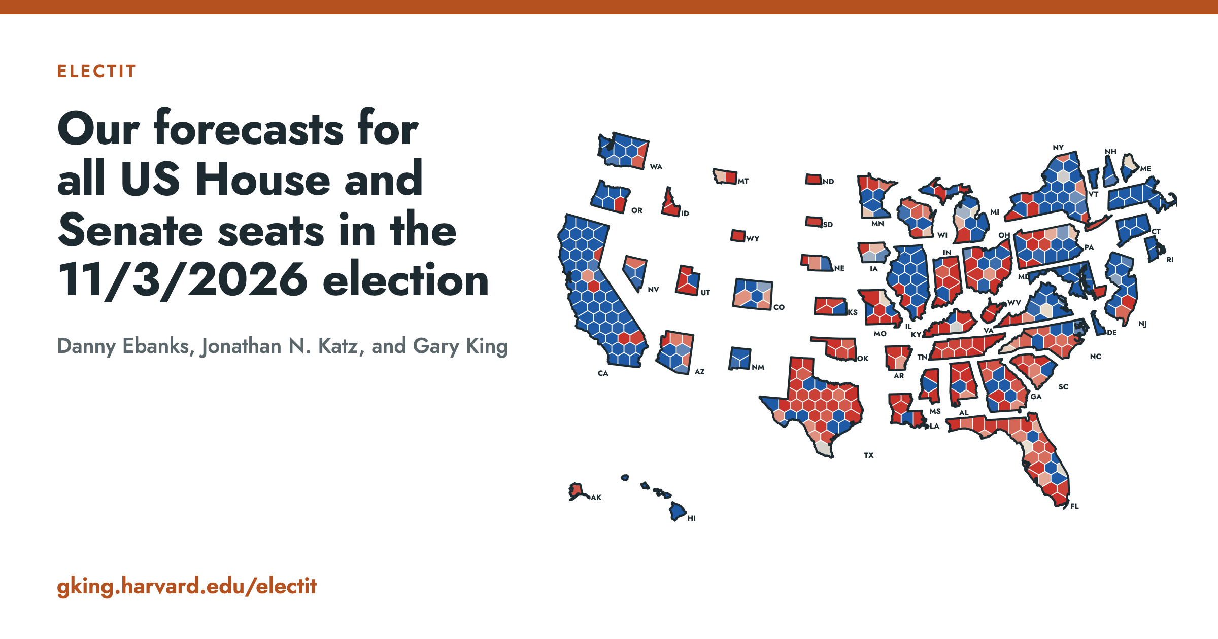
ElectIt · U.S. elections forecast
We evaluate elections probabilistically. That means we assign probabilities to events before they happen. If we assign a 10% chance that a Republican wins, we expect they should win 10% of the time.
This means that for the model to be proven wrong, we need to look at the big picture, not any one election or quantity. So, when we aggregate all the events that we assigned 10, 20, and 30% probabilities, those events should occur at roughly that rate.
If the model makes no mistakes, our probabilities were underconfident. If the model makes too many mistakes, it is overconfident.
The model says there’s a – chance the Democrats take the House
Loading the forecast…
- Forecast Democratic House seats–
- Seat Changes–
- National House vote, Democratic –
- Competitive seats–
No districts called yet.
435 House districts
Republican winevenDemocratic win
Model-Informed Analysis
Here are five scenarios that are informed by our Model + All Polls forecast, historical polling error, and the latest polling data.
If the Polls Are Largely Correct
The polls are exactly right (with 0.13 probability, the national vote is within half a point on margin of our forecast)
The polls are largely correct, in line with historical performances in 2022, 1994, and 1990. The quantitative forecaster consensus, prediction markets, national polls, district and state polls, and the fundamentals models (which all largely agree on the direction and magnitude of the national trend) are correct in their assessment of the campaign, which is that this is a standard midterm election where the president’s party loses ground in the legislature. Given the relatively Democratic-leaning environment and strong candidates, Democrats overperform the political geography in the Senate and gerrymandering efforts in the House, and go on to win the House with a large majority of roughly 240 seats and win states that lean Republican in a neutral political environment, like Alaska and Texas. They also win either Iowa (a reaction to tariffs) or Kansas, with a strong candidate in Adam Hamilton ().
The national vote is in line with our model’s expectations, within a quarter point of the 54.1% share we expect for the Democratic Party (half a point on margin). In this scenario (probability 0.13), Democrats win both the House and the Senate with 0.83 probability. The median forecast is 239 House seats and 52 Senate seats. Since 1950, the median polling error is 2 points in either direction, and 3 of the 19 midterms have had an error within 0.5 points (1990, 1994 and 2022). Polls as accurate as in those years would be enough for this type of result.
Model-Informed Analysis
The snake
Each box represents a seat, shaded by which party our model thinks is favored. A bold outline indicates a party flip.
Most likely tipping points
Seats Most Likely to Flip
How Votes Become Seats
House Odds If the Polling Average is the Same on Election Day
Distribution of Margins Across Seats
The Math Behind the Forecast
We iteratively make three forecasts, with each building on the others in successive order. The Post-Nomination Forecast is LogisTiCC. Model + Generic Ballot weights the model’s simulations by the national generic-ballot polls, by providing a Bayesian update to the national trend and the fundamentals. Model + All Polls then adjusts our simulations from LogisTiCC given district and state polls. We then use these polls to further adjust the national trend.
1. The Post-Nomination Forecast: the LogisTiCC model
The 2026 elections. We forecast all House districts using their 2026 district lines (nine states redistricted since 2024). Candidates and incumbents are as of October 1, 2026. Louisiana chooses its House nominees on November 3, so its six seats assume the incumbents run. We treat an election with multiple candidates from the same party as uncontested. We treat Kevin Kiley, who runs as an independent in CA-6, as a Republican for the purposes of this forecast. We forecast 35 contested Senate seats, noting that for a majority, Democrats will need 51 seats to beat the Vice President’s tiebreaking vote.
The model. We build on the standard linear-normal model of district-level elections, keeping the same flexibility in the choice of covariates within a fully Bayesian framework. We designed each feature of the model using the field’s knowledge of elections, adding “known unknowns” that reflect what students of elections understand well but rarely model directly. We call the result LogisTiCC, for the additive logistic t model with contemporaneous correlations. It fits every House and Senate election of 1946–2024 from one data generation process. The outcome variable is the Democratic proportion of the two-party vote, vit, for district i (a state, in the Senate) and election year t:
logit(vit)=μit+ωit,ωit∼tνit(0,ϕit)
μit=Xitβt+γD(i,t)−γR(i,t)+ηt
ϕit=exp(ζ+ζd+Zitδ),νit=1+exp(α+αd+Zitλ)
Our structural covariates, Xit, are the election’s past results (its own lagged effective vote and the district’s lagged presidential, Senate, and governor votes), incumbency, open seats left involuntarily or by a strategic exit, the South, an uncontested election, and a midterm penalty, which represents the strong tendency of the president’s party to lose ground in midterm elections. Their slopes, 𝛽t, show parameter drift with coefficient stability: they vary a lot in the long run but change very little from year to year, so each follows a random walk, 𝛽tk ∼ N(𝛽t−2,k, 𝜎𝛽k2).
The candidate effects, 𝛾D(i,t) and 𝛾R(i,t), model candidate uniqueness. They are person-specific intercepts on the Democratic and Republican candidates in the election, drawn from a common distribution, 𝛾c ∼ N(0, 𝜎𝛾2). Each is the candidate’s valence net of party, incumbency, the district’s partisan lean, and the model’s other systematic components, and an election in which one major party fields no candidate drops that party’s term.
The national trend, 𝜂t, allows for positive cross-district covariances: it affects all districts in one election in roughly the same way, over and above the information in X. It models the familiar observation that some years are good for Democrats and others for Republicans, even if we do not know which is which ex ante: 𝜂t ∼ N(0, 𝜎𝜂,d(t)2), its standard deviation estimated for each redistricting decade, d(t). In midterm years, we also account for year-to-year variation in the midterm penalty, as the generic ballot provides information about both 𝜂t and the midterm penalty.
The error, 𝜔it, models district-level political surprises. We use the additive logistic Student t (ALT), which, unlike the normal, constrains the vote proportion to the (0,1) interval and has appropriately fatter tails to represent surprises, with more of its density concentrated near the mean. Its scale, 𝜙it, and degrees of freedom, 𝜈it, depend on Zit: an open-seat indicator, the marginal distance from 50/50 in the district’s lagged presidential vote, and an indicator for single-district states and the Senate, with slopes 𝛿 and 𝜆, intercepts 𝜁 and 𝛼, and redistricting-decade effects 𝜁d and 𝛼d. Safe seats’ future vote shares are relatively predictable from one election to the next, whereas a competitive seat exhibits a far greater tendency to surprise.
We formally distinguish between the observed vote, vit, and the effective vote, vit*, the vote proportion that would have been observed if the election had been contested. We estimate the unobserved effective votes as unknown parameters with all the others, under a censoring assumption: candidates running unopposed would have won even if the election were contested.
The forecast. Each of the 160,000 simulations draws the model’s parameters from their posterior, then 2026’s national trend, 𝜂, from N(0, 𝜎𝜂2) with the 2020s’ 𝜎𝜂, then every election. With equal weights, the simulations are the Post-Nomination Forecast: an election’s chance is the frequency with which the Democratic candidate wins in our simulations, and the chance of a Democratic House is the share in which Democrats win 218 or more seats.
2. Model + Generic Ballot
Our model, LogisTiCC, simulates each House and Senate election times. As reported in our paper, we estimate a national trend, 𝜂, which shifts every election in a given year in logit space by the same magnitude. Model + Generic Ballot keeps every simulation and gives each one a weight. A simulation counts more when its national House vote agrees with the most recent observed value of the generic ballot. We build it in eight steps.
-
Compute each simulation’s national vote. A simulation’s national vote, V, the Democratic share of the two-party House vote, is:
V(η)=∑iTilogit−1(ci+η),ci=Xiβ+γD(i)−γR(i)+ωi
Here i is a district, and ci is election i‘s logit without the national trend: its fundamentals, its candidates, and its surprise. The inverse logit, logit−1(x) = 1/(1 + e−x), turns a logit back into a share. To replicate the official count of the popular House vote, our estimated national vote is weighted by how many votes we expect to see in each district, which we measure by Ti, its share of ‘s presidential turnout, with each unopposed seat at its recorded share. In the unopposed elections of 1946–2024, the official count recorded 66% as many votes for their turnout as in contested elections (33% in Florida, which recorded no votes for half of them, and 81% in California). We estimate turnout based on current district lines, calculated using precincts from 2014–2024, and county-level returns from 1946–2012. Ti is not a known parameter: it is a forecast, and the House electorate it stands in for changes from year to year. So we add one-step-ahead forecast noise to it (step 5), estimated from all election results prior to the forecasted year: now points of the national vote.
-
Incorporate a tied-election baseline. To allow for more effective simulations in the Build Your Own modeling feature, we augment the tails of the prior distribution (our LogisTiCC forecast). We shift each simulation’s national trend by Δ = , toward the . This shift makes Democrats win 218 or more seats in exactly half of the set of effective simulations. We call this set of simulations the Tied House Election Baseline, and their average national vote is %. This allows us to explore parts of the simulation space far away from what the model expects after the primary. This is especially helpful if there are large shifts in the fundamentals over the course of the campaign. We then sample from the mixture of these two normal distributions:
q(η)=12N(η;0,ση2)⏟the model’s prior: the simulations+12N(η;Δ,ση2)⏟the prior shifted by Δ: the Tied House Election Baseline
Here 𝜎𝜂 is the model’s standard deviation for the national trend. The mixture only supplies draws. Step 7 counts each draw by the model’s own prior for 𝜂, so if the generic ballot holds no useful information, the forecast returns to the Post-Nomination Forecast.
-
Fit a regression line that predicts the generic ballot from the national vote. We fit a regression of the generic ballot on the official national vote, using . For previous forecasts, we only use data available prior to that specific election. We use the final generic-ballot margin, G, and the national House vote, V.
G=a+b⋅logit(V)+e,e∼N(0,σG2)
Here a is the intercept, b is the slope on the logit of V, and e is the poll’s error, with standard deviation 𝜎G. We estimate the regression line by weighted least squares:
a^=,b^=,σ^G=
National polling errors have decreased since the , so we allow the size of errors to drift over time, from in the to in the . For each holdout forecast prior to 2026, we estimate this regression for midterms and presidential elections separately. We only estimate the national vote once we have at least 5 years’ worth of data points in each regression. Since we do not observe 5 midterm and 5 presidential elections prior to 1958, we pool both midterms and presidential elections together to estimate the above regression (as we have generic ballot estimates going back to 1938) for 1948–1956.
Polls have become more accurate, so we count recent midterms more, at nine possible rates, 𝜆, from 1 (all midterms count the same) to 0.5. We weight each rate by how well it predicted the generic ballot in each earlier midterm, using only the elections before that midterm. .
Steps 4 to 7 run once with each rate’s regression line. Step 7 then averages the draws’ weights over the rates. Each regression line uses its own σ^G. A polling error that you set applies to every regression line whose σ^G is smaller. The figures that we show for the regression line, such as its intercept, its slope, σ^G, and k of step 4, are the best rate’s.
-
Compute the likelihood of the most recent observed value of the generic ballot. For a simulation with national vote V, the regression line predicts the generic ballot. The likelihood of the most recent observed value of the generic ballot is
L(G|V)=N(G;a^+b^⋅logitV,kσ^G2)
We employ a small sample correction for the variance, as we are estimating regression parameters on so few elections. It is the standard small-sample correction for a prediction from an estimated regression:
k=(1+1+(logitV)2)
For more information, see here: Gelman, Carlin, Stern, Dunson, Vehtari, and Rubin, Bayesian Data Analysis, 3rd edition (2013), Section 14.2.
-
Update each simulation with the generic ballot. Each simulation, s, is sampled from a posterior distribution based on the fundamentals, 𝜃s (its candidates, districts, and the model’s other parameters), and the national trend, 𝜂s. The generic ballot provides information about how both fundamental and the national trend may have shifted since the primary. Applying a Bayesian update when the model learns the generic ballot, we can decompose the posterior distribution into two components:
p(θ,η|G)∝p(θ)⋅N(η;0,ση2)⋅L(G|V(θ,η))=p(θ|G)⋅p(η|θ,G)
The first component reweights the simulations by increasing weight to simulations whose fundamentals are implied the generic ballot results we actually observe. The second component is the national trend implied by the generic ballot and this updated set of fundamentals:
p(θs|G)∝Zs,Zs=∫N(η;0,ση2)L(G|V(θs,η))dη≈N(xG;αs,ss2+τ2)
where xG is the logit transformation of the national vote, 𝛼s and ss are the mean and variance of simulation s‘s national vote, and 𝜏2 is the generic ballot’s prediction variance. Simulations whose fundamentals are consistent with scenarios that are implied by the current observation of the generic ballot are given increased weight. When the generic ballot and the fundamentals strongly disagree, the forecast will assign increased probability to scenarios that are consistent with the generic ballot rather relative to the fundamentals.
First, we assume that the generic ballot’s residual error is uncorrelated with the national trend. Second, we assume the generic ballot is only related to individual elections through the national trend. We then convert the generic ballot into logit units, to make it comparable to the national trend, 𝜂, which is also expressed in logits.
- We invert the regression line. This gives the national vote that the most recent observed value of the generic ballot implies, logitVG=(G−a^)/b^: % at .
- Within a simulation, the logit-transformed national vote is approximately linear in the national trend, logitV(η)≈y0+βη. Here y0 is its value with no national trend, and 𝛽, about , is how far it moves for each unit of national trend. 𝛽 is less than one, because elections far from 50–50 change their share of the vote less. The national trend that moves the simulation’s national vote to VG is ηG=(logitVG−y0)/β.
- The regression line’s prediction error goes with it: 𝜂G has variance (kσ^G2+b^2σT2)/(b^β)2. We divide the regression line’s variance by b^2 to put it on the logit of the national vote, and by β2 to put it in the national trend’s units, with k at VG. The turnout weights, Ti, are a forecast too, so the variance also carries their one-step-ahead error, 𝜎T, on the logit of the national vote: how far the national vote under Ti ran from the official count in the elections before the year, with a t‘s small-sample correction ().
The model’s prior for the national trend, N(0, 𝜎𝜂2), and the trend implied by the generic ballot, 𝜂G, combine into a normal update with mean 𝜂1 and variance 𝜏12:
1τ12=1ση2+(b^β)2kσ^G2,η1=τ12(b^β)2ηGkσ^G2
The smaller the polling error is against the model’s spread for the national trend, 𝜎𝜂, the more strongly the forecast moves toward the generic ballot’s trend.
-
Allow the posterior uncertainty in 𝜂 to shrink as Election Day approaches. By Election Day, the average can still move by the drift, and the vote can differ from it by any polling error that you set above σ^G:
τ22=τ12+drift2+k(σ2−σ^G2)(b^β)2
The update’s center, 𝜂1, stays where step 5 put it. Only its variance grows. Uncertainty in our model, whether due to forecasting the election result earlier in the election cycle or due to larger estimated polling error (which is driven upwards when constituent pieces of the data give conflicting signals), is hedged towards a toss-up election. On Election Day at the historical error, 𝜏22 = 𝜏12.
-
Reweight the Post-Nomination Simulations. We then reweight the simulations by importance sampling. The intuition behind this second reweighting is that given new information in the form of the Generic ballot (), we ask how likely this observation is taking the national vote as given, alongside the regression error structure and polling drift we estimated above. Simulations whose national vote is near %, i.e., the ones most consistent with , get the most weight. We weight every simulation, including the Tied House Election Baseline, so that they all jointly follow the updated posterior for 𝜂. In the chart, the shaded areas show where the 320,000 simulations fall on the national vote: the model’s simulations below and the Tied House Election Baseline above. The gray dashed line outlines them all. The gold line is the Model + Generic Ballot’s best estimate for the national vote. We give more weight to simulations where the gold line rises above the distribution outlined by the gray dashed line, and less to simulations where it falls below the gray dashed line. On average, a simulation’s weight is the gold line’s height over the dashed line’s height at its national vote. The chart starts at your settings. Move the four settings here to watch the weights change; the forecast above stays as it is.
Now, each simulation will be drawn with national trend 𝜂s, from the mixture distribution q we derived in step 2. The forecast needs each simulation’s national trend to be drawn from the implied posterior distribution given a user’s settings, p(𝜂 | 𝜃s, G, 𝜎, drift), and each simulation to count by Zs, the first component of step 5. So each draw’s weight is Zs times the ratio of the two densities, for its fixed national trend:
ws=Zs⋅p(ηs|θs,G,σ,drift)q(ηs)
That distribution is the update of steps 5 and 6:
p(η|G,σ,drift)={N(η;0,ση2)L(G|V(η))Con Election Day, σ=σ^GN(η;η1,τ22)otherwise
On Election Day at the historical error, nothing widens the update, so it is step 5’s p(𝜂 | G). Here C, the normalizing constant, is the marginal likelihood of the most recent observed value of the generic ballot under each simulation’s prior for the national trend:
C=∫−∞∞L(G|V(u))N(u;0,ση2)du
C is step 5’s Zs, so on Election Day the two cancel, and a draw’s weight is the model’s prior times the likelihood over q: we weight a simulation more heavily if the observed generic ballot result is more likely given that simulation’s fundamentals and draw of the national trend. With days left or a larger error, p is the normal update, widened in step 6, and Zs is its normal approximation of step 5. We reweight because reweighting is fast and stays stable when the settings describe a campaign that the model finds unlikely.
Each rate’s regression line of step 3 gives draw s its own weight, ws(𝜆), by the ratio above. The forecast’s weight for the draw is their weighted average, with the rates’ weights, 𝜋𝜆:
ws=∑λπλws(λ)
-
Count the seats. The weighted simulations are then summed to calculate Model + Generic Ballot’s seat predictions and probabilities, and the election polls then move each polled election to give Our Forecast. In draw s, election i‘s Democratic share is vis=logit−1(cis+ηs). An election’s forecast vote share and its chance of a Democratic win are weighted averages over the 320,000 draws:
v^i=∑swsvis∑sws,Pi=∑sws1[vis>0.5]∑sws
The chance of a Democratic House is the sum of the weights of the draws in which Democrats win 218 or more seats, divided by the sum of all the weights. The Senate’s chance uses the draws with 51 or more Democratic seats, because the vice president is a Republican. The expected seats and their ranges come from the same weights. Beyond a 10-point polling error, the draws no longer span the range of outcomes, so the error box stops at 10.
Why reweighting gives the same answer as resampling. We draw our simulations from a modified (and deliberately biased) distribution q, which has more probability mass in the tails than the LogisTiCC prior, which we call 𝜋. The target distribution, p, is the LogisTiCC prior 𝜋 multiplied by the likelihood of the observed generic ballot given the national trend (which we calculate from a regression), normalized to integrate to one. In importance sampling, we then calculate a weight for each draw, w = p/q. So a simulation in a region where q has extra mass is weighted proportionally less, and a simulation in a region that q undersamples is weighted more heavily. For any quantity of interest h, such as the number of Democratic seats or an indicator function for the event that Democrats win (from which we calculate the probability of the Democrat wins), the weighted expectation of h is
Eq[h⋅pq]=∫h⋅pq⋅qdη=∫h⋅pdη
The trick is that the sampling distribution q cancels in this expression, so the weighted average has the same expectation as an unweighted average of draws from our posterior, p. If we normalize the weights so that they sum to one, the estimate has a small Monte Carlo bias that shrinks at the rate 1/(effective number of draws). We have draws, and at generic ballot about of them are effective, so this bias is far smaller than the ordinary simulation noise.
3. Model + All Polls
We build our Model + All Polls model by starting with our Model + Generic Ballot model as a foundation. Individual polls affect their specific districts. We allow them to share a correlated error with the generic ballot polling as well, which we estimate from historical polling performance. A margin is the Democrat’s two-party share minus the Republican’s, in percentage points. We proceed to incorporate individual polls in the six following steps.
-
Calculate a Polling Average for Each State or District Election. The average for election j, ȳj, is the weighted mean margin of its nj polls: every poll from the nominations to , from ; now . Each poll counts half as much for every days of age, the half-life that best predicted the elections before the year. Poll k is ℓjk days old, its margin is yjk, and its weight is 𝜅jk:
y¯j=∑k=1njκjkyjk∑k=1njκjk,κjk=2−ℓjk/14
We adjust polls sponsored by partisan organizations ().
-
Model Correlated Polling Errors. We decompose polling error for a single district or state election, mj, in five mean-zero components. We assume the polls do not systematically favor one party or another over time.
y¯j=mj+ξ+ρg(j)+ςS(j)+uj+ej
ξ∼N(0,τnat2),ρg∼N(0,τreg2),ςS∼N(0,τstate2)
uj∼N(0,σrace2),ej∼N(0,σpoll2njeff)
Here 𝜉 is a national component that the year’s elections share, 𝜌g(j) is a regional component that the elections of Census region g(j) share, 𝜍S(j) is a state component that the elections of state S(j) share, uj is its individual election component, and ej is a sampling component that shrinks with the polls’ effective number, njeff=(∑κjk)2/∑κjk2. So the averages’ errors have covariance
Rjk=τnat2+τreg21[g(j)=g(k)]+τstate21[S(j)=S(k)]
+1[j=k](σrace2+σpoll2njeff)
where 1[·] is an indicator function. We add the state component because polls of elections in one state err together. In our polls within 20 days of the election, House and Senate elections in the same state shared an error beyond the national and regional errors. Over the 310 state-years of 1990–2024 with two or more polled elections, its standard deviation was about 2.5 points. Before 1990, the polls are too few to measure it. With the state component, polls of several districts in one state cannot confirm each other at full strength. In each simulation, the House and the Senate share one draw of the national, regional, and state components. Each chamber scales that draw by its own sizes. So a state’s Senate polls and its House district polls err together.
All of an election’s polls share these components, so several old polls in one election cannot average that error away. The sizes are:
-
Adjust Simulations to Account for Election-Level Polling Averages. For each simulation, s, we adjust the simulation by ms using an ensemble Kalman gain, K:
ms′=ms+K(y¯+εs−ms)
εs∼N(0,R),K=D(D+R)−1
Here D contains each polled election’s variance across the weighted simulations, and R is the error covariance of the polling averages from step 2. In each simulation, we add its own draw of the polling error, 𝜀s, to the polling averages. As a consequence, the adjusted simulations keep the spread that the polling error leaves. The polls of many elections can err together, and R includes the national, regional, and state components that they share. So we adjust each election less when many polling averages differ from a simulation in the same direction than when one average differs alone. The elections without a published poll stay where Model + Generic Ballot left them, and every simulation keeps its weight.
The district and state polls can err together with the generic ballot. So we let the national component of their error, 𝜉, correlate with the generic ballot’s error. We estimate this correlation, r, for each year and chamber from pairs of errors in the elections before that year. We set r to n/(n + 10) times the correlation of the n pairs, which shrinks r toward zero most when the pairs are few. When there are fewer than five pairs, we set r to zero.
The first error in each pair is the generic ballot’s error in an earlier election. This error is the final G minus the margin that the election’s own regression line predicts from its national House vote, averaged over the rates. The second error is the national component of the error of the district or state polls on the eve of that election. We estimate that component with the error model of step 2.
In simulation s, the generic ballot’s error is es. From the most recent observed value, it has standard deviation 𝜎tot, and its correlation with the national component, 𝜉, is reff:
es=G−(a^+b^⋅logitVs),σe2=kσ2
σtot=σe2+drift2,reff=rσeσtot
Here Vs is the simulation’s national vote. The regression line, k, the polling error 𝜎, and the drift are those of Model + Generic Ballot (steps 3 and 4, and the settings of Build Your Own below), with the regression line at the best rate and k at VG. 𝜎e2 is then the variance of the regression line’s prediction. Only the polling error in es is correlated with the district and state polls. The drift is not. So reff scales r down by 𝜎e/𝜎tot. Election j‘s average then has an expected shared error, 𝛿s,j. The national component keeps the variance that remains, so R becomes R′:
δs,j=reffτnat,jesσtot,Rjk′=Rjk−reff2τnat,jτnat,k
Here 𝜏nat,j is 𝜏nat of step 2 at election j‘s distance, so the national term of Rjk is 𝜏nat,j𝜏nat,k. With the correlation, the update becomes:
ms′=ms+K(y¯−δs+εs−ms)
εs∼N(0,R′),K=D(D+R′)−1
Here 𝛿s holds the elections’ 𝛿s,j. With r = 0, it is the update above. Where the generic ballot overstates the Democrats in a simulation, we read the district and state polls as overstating them by a share of that. Where it understates them, we read the district and state polls as understating them by a share of that. Both kinds of polls can err together, so they should not confirm each other at full strength.
-
Allow for correlations between the National Trend and Individual Polls (the District and State Poll Trend Adjustment): When we adjust the district-level results based on polls in the previous step, our model assumes that a Democratic overperformance across many districts is indicative of polling error. We allow for that, but in this step, we also allow that it is a signal of a potential shift in the national trend. We then decompose how much of the difference in district-level polling from our generic ballot model is due to polling error versus real shifts in the polls based on historical polling performance. The polls’ common gap, x¯, is the weighted average distance of the polled elections’ averages, y¯j, from Model + Generic Ballot’s mean margins, m^j. An election’s weight, gj, is larger when its average is more precise. The weights sum to one:
x¯=∑jgj(y¯j−m^j),g=(D+R)−111T(D+R)−11
Here D and R are those of step 3, and 1 is a column of ones. We then adjust the national trend in every simulation by the same amount, Δη. Each election moves by its own response to the national trend, βi: the slope of its margin on 𝜂 across the weighted simulations. Δη moves the polled elections’ weighted average margin by 𝜓x¯:
ms,i″=ms,i′+βiΔη,Δη=ψx¯∑jgjβj
Using only earlier elections, we estimate 𝜓, the historical amount of the gap between the district polls and Model + Generic Ballot that is due to genuine changes in the national trend. The rest of this difference is treated as non-systematic polling error. A year with fewer than five earlier elections with polls, as before 1978, has 𝜓 = 0. In the Senate, every contested election moves. In the House, districts with polling data are adjusted, but for those with no polls, we report the Model + Generic Ballot forecast for that district.
ψ=min(1,max(0,∑t<Yx¯t(r¯t−u¯t)∑t<Yx¯t2))
We estimate 𝜓 separately for the House and the Senate, for each week before the election. For a day between two weeks, we interpolate linearly between their estimates. Here t is an earlier election with polls recorded at the same time before Election Day. For election t, x¯t is the polls’ common difference from the Model + Generic Ballot forecast, u¯t is the weighted average of the step 3 adjustment to the elections with polling data, and r¯t is the weighted average of the difference between the results and Model + Generic Ballot. All three use the weights g of election t.
-
Count the seats in each simulation, as in Model + Generic Ballot.
-
How we model Previous Years’ Polling Errors. If you select a polling-error scenario for a previous year, we assume that the estimates from the error model for that year are then given, including region and national polling error. We allow the individual state and district election error and sampling error components to remain random:
y¯j−ξ^Y−ρ^Y,g(j)
Rjk=τstate21[S(j)=S(k)]+1[j=k](σrace2+σpoll2njeff)
Why we move the simulations instead of reweighting them. Reweighting the simulations by every district’s and state’s polls at once leaves too few: in 2018’s House, one effective simulation of 40,000. This approach allows us to shift the individual elections without decreasing the number of effective simulations. Letting the polls move every election through the simulations’ full covariance did worse in the holdouts when the polls erred together, as in 2016 and 2020.
Build Your Own
For Build Your Own forecasts, we let you select your own values for the generic ballot (or use RCP’s or Silver Bulletin’s), we let you select the variance of the polling error, we let you select how much the polls might change from now until Election Day. You can also choose to include, exclude or modify candidate effects. Finally you can also see how the forecast changes if the polls are biased as they were in previous elections from 1960 to 2024.


